Analog Signal Chains: Infrastructure for Sensors and Industry

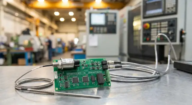
What an analog signal chain is (and why it matters)

An analog signal chain is the set of circuits that takes a real-world quantity—like temperature, pressure, vibration, or light—and turns it into a clean, scaled electrical signal that a system can reliably use. That system might be a microcontroller reading an ADC value, a PLC input module, a handheld meter, or a lab instrument logging data.

The core idea is simple: before you ever see a number on a screen, you’re handling physics. The signal chain is the infrastructure that bridges messy reality and usable data.

Why measurements start out analog

Most sensors interact with the world in continuous ways. Heat changes resistance, strain changes a bridge imbalance, light generates current, motion induces voltage. Even when a sensor exposes a digital interface, the sensing element inside is still analog—and someone designed a chain around it.

Analog sensor outputs also tend to start small and imperfect: microvolts from a thermocouple, tiny currents from a photodiode, millivolt-level bridge outputs from load cells. Those signals ride on offsets, noise, cable pickup, and power-supply ripple. Without conditioning, the “data” you collect can end up reflecting your wiring and electronics more than your process.

Where analog signal chains show up

You’ll find them anywhere measurement quality matters:

• Factories and industrial automation: pressure and flow transmitters, motor monitoring, safety systems, high-noise environments with long cables.
• Instruments and lab equipment: balances, oscilloscopes, data acquisition (DAQ), precision temperature control.
• Vehicles and machines: battery monitoring, current sensing, vibration sensing, engine/drive control feedback.

Practical trade-offs, not theory

Signal-chain design is less about textbook-perfect circuits and more about informed compromises: accuracy vs. cost, bandwidth vs. noise, power vs. performance, and “good enough” vs. “auditable.” The goal is trustworthy measurements under real constraints.

The building blocks you’ll see in this post

A practical analog signal chain typically includes sensor excitation/biasing, amplification and conditioning, filtering for noise and interference, ADC selection, voltage references and calibration, power management, and isolation/protection for the real world. Each block affects the next, so treating the chain as a system is how you avoid expensive surprises later.

From sensors to signals: what you’re really measuring

A sensor doesn’t hand you a clean “temperature = 37.2°C” value. It produces an electrical effect that correlates with a physical quantity—and your job is to preserve that correlation through the analog signal chain.

What sensors actually output

Common industrial sensors tend to fall into a few output types:

• Millivolts (mV): thermocouples, some piezoresistive bridges
• Microamps to milliamps (µA/mA): 4–20 mA transmitters, photodiodes (often µA)
• Resistance (Ω): RTDs, thermistors, strain gauges (as part of a bridge)
• Charge (pC): piezoelectric sensors (often converted with a charge amplifier)

These are rarely “plug into an ADC” signals. They’re small, sometimes fragile, and often riding on offsets or common-mode voltages.

Ranges, headroom, and real-world ugly bits

Real measurements include tiny signals plus large offsets, plus spikes from switching loads, ESD, or nearby motors. If your amplifier or ADC runs out of headroom—even briefly—you can clip, saturate, or take seconds to recover.

Sensors also have imperfections you must plan for: drift with time/temperature, nonlinearity across the measurement span, and hysteresis where the output depends on whether the input is rising or falling.

Source impedance: the “hidden” specification

Source impedance describes how strongly the sensor can drive the next stage. A high-impedance source (common with certain probes and charge outputs) can be distorted by input bias currents, leakage, cable capacitance, or ADC sampling kickback. Buffering and input filtering aren’t optional—they often determine whether you’re measuring the sensor or your circuit.

Example: thermocouple vs. RTD vs. strain gauge

A thermocouple might produce only tens of µV/°C, demanding low-noise gain and cold-junction compensation. An RTD is a resistance that needs stable excitation and careful lead-wire error handling. A strain gauge typically lives in a Wheatstone bridge, producing mV/V changes that require an instrumentation amplifier and attention to common-mode range.

The building blocks of a practical signal chain

A practical analog signal chain is the path from “something happening in the real world” to a number you can trust in software. Most systems reuse the same blocks, even if the sensor type changes.

A typical chain (in plain terms)

1. Excitation / biasing: some sensors need a stable current or voltage to operate (or a bias point to center an AC signal).

2. Front-end / conditioning: buffering, level shifting, and often an instrumentation amplifier to boost tiny signals while rejecting common-mode noise.

3. Filtering: analog low-pass (and sometimes notch) filtering to prevent out-of-band noise and aliasing.

4. Conversion (ADC): turning voltage into digits with the required resolution, sample rate, and input range.

5. Reference + calibration: a stable voltage reference and a way to correct gain/offset errors over time and temperature.

6. Processing: digital filtering, linearization, diagnostics, and data packaging for the rest of the system.

Let the measurement spec drive the design (backwards)

Start with what the output must mean—accuracy, resolution, bandwidth, and response time—then work backward:

• ADC resolution is meaningless if front-end noise is higher than one LSB.
• A great amplifier won’t help if the reference drifts with temperature.
• A clean schematic can still fail if the sensor cable picks up interference.

Why “good enough” breaks at scale

A single-channel prototype may pass, but 32 or 128 channels expose issues: tolerances stack up, channel-to-channel matching matters, power and grounding get crowded, and service teams need repeatable calibration.

Early requirement checklist

• Sensor type, full-scale range, and expected fault states
• Required accuracy (including temperature range) and update rate
• Cable length/environment (EMI, ESD, surges)
• Channel count, board area, cost target, and calibration strategy
• Serviceability: test points, self-checks, and replacement procedure

Sensor excitation and biasing: starting with a stable foundation

Most real-world sensors don’t “generate a voltage” on their own. They change a resistance, current, or light level, and your job is to provide a known electrical stimulus—excitation or bias—so that change becomes a measurable signal.

Why excitation is required

• Strain gauges and load cells (Wheatstone bridges) need a stable bridge voltage (or current). The sensor’s output is a tiny difference voltage proportional to load.
• RTDs are resistors whose value tracks temperature, so you typically drive them with a precision current source and measure the resulting voltage.
• Optical sensors often require LED drive current. The LED intensity is part of the measurement, so its stability directly affects accuracy.

What “stable” really means

Excitation isn’t just “the right value”—it must stay consistent across time and temperature. Low noise and low drift matter because any wobble in excitation looks like sensor movement.

Temperature effects show up in multiple places: the reference that sets your current/voltage, resistor tempco in the current source, and even PCB leakage at high humidity. If the system must hold calibration for months, treat the excitation circuit like a measurement channel, not a utility rail.

Ratiometric measurements (simple version)

A practical trick is to measure the sensor output relative to the same excitation powering it. For example, using the bridge excitation as the ADC reference means that if excitation shifts by 0.5%, both numerator (signal) and denominator (reference) shift together—so the final reading barely changes.

Multiplexed systems and common pitfalls

When many channels share excitation (vs. per-channel), watch for loading changes and settling time after switching. Long cables add resistance and pickup; RTDs suffer lead resistance unless you use 3‑wire/4‑wire connections. Finally, don’t ignore self-heating: more excitation current improves signal size but can warm an RTD or bridge and quietly bias the measurement.

Amplification and conditioning: making tiny signals usable

Sensors often produce signals that are small, offset, and riding on top of electrical junk from motors, long cables, or power supplies. Amplification and conditioning is where you turn that fragile sensor output into a clean, correctly sized voltage that your ADC can measure without guesswork.

Instrumentation amplifier vs. low-noise op-amp

Use an instrumentation amplifier (in-amp) when you’re reading a differential signal (two wires from the sensor) and you expect cable pickup, ground differences, or a large common-mode voltage. Classic examples are strain gauges, bridge sensors, and low-level measurements far from the electronics.

A low-noise op-amp is often enough when the sensor output is single-ended, the wiring is short, and you mainly need gain, buffering, or filtering (for example, a photodiode amplifier or a conditioned 0–1 V sensor).

Gain setting: the silent trade-off

Gain should be chosen so the largest expected sensor signal lands close to the ADC’s full-scale range—this maximizes resolution. But gain also amplifies noise and offsets.

Two failure modes show up repeatedly:

• Saturation/clipping: a slightly larger-than-expected input (or a startup transient) pushes the amplifier to the rail, flattening peaks and ruining readings.
• Noise dominance: too much gain can amplify broadband noise so much that it becomes the limiting factor, even if your ADC is excellent.

A practical rule is to leave headroom for tolerances, temperature drift, and rare but real events like sensor faults.

Common-mode voltage and CMRR (an intuitive example)

Imagine a bridge sensor produces a tiny 2 mV change, but both wires sit at about 2.5 V because of the biasing. That 2.5 V is the common-mode voltage.

An in-amp with high CMRR (common-mode rejection ratio) mostly ignores that shared 2.5 V and amplifies only the 2 mV difference. Low CMRR means that “shared” voltage leaks into your measurement as error—often looking like drift or inconsistent readings when nearby equipment switches on.

Input protection and layout sensitivity

Inputs should survive real life: ESD, accidental overvoltage, reversed connections, and miswiring. Typical protection includes series resistors, clamps/TVS diodes, and ensuring the amplifier’s input stays within its allowed range.

Finally, tiny signals are layout-sensitive. Leakage currents across dirty boards, input bias currents, and stray capacitance can create phantom readings. Techniques like guard rings around high-impedance nodes, clean routing, and careful connector selection are often as important as the amplifier choice.

Noise, interference, and filtering: keeping measurements clean

A sensor signal chain doesn’t just carry a measurement—it also picks up unwanted signals along the way. The goal is to identify what kind of error you’re seeing, then choose the simplest fix that preserves the information you care about.

Where noise comes from

Thermal (Johnson) noise is the unavoidable hiss from resistors and sensor elements. It increases with resistance, bandwidth, and temperature. 1/f (flicker) noise dominates at low frequencies and can matter in slow, high-gain measurements (like microvolts from strain gauges).

Then there’s interference: energy coupled from the environment, usually periodic or structured. Common culprits are 50/60 Hz mains (and its harmonics), motor drives, relays, and nearby radios.

Once you digitize, you’ll also see quantization noise from the ADC: the stair-step error due to finite resolution. It’s not a wiring problem, but it can set the floor for how small a change you can reliably see.

Random noise vs. periodic interference

A useful rule: random noise broadens your readings (they jitter), while periodic interference adds a recognizable tone (often a stable ripple). If you can spot it on an oscilloscope or in an FFT as a narrow peak at 50/60 Hz, treat it like interference, not “bad sensor noise.”

Filtering choices that actually help

• RC low-pass filters are cheap and effective for slow signals.
• Active filters (op-amp based) give sharper roll-off when you need to keep more bandwidth while rejecting out-of-band noise.
• Anti-aliasing filters are essential before an ADC: any energy above half the sampling rate can fold into your measurement as false content.

Bandwidth should match the physics: a temperature probe might need a few Hz; vibration monitoring may need kHz. Over-wide bandwidth makes noise worse for no benefit.

Practical wiring tips

Use twisted pair for differential signals, keep loops small, and place the first amplifier close to the sensor when you can. Prefer a clear grounding strategy (often single-point for sensitive analog) and avoid mixing high-current returns with measurement grounds. Add shielding when you must—but bond the shield thoughtfully to prevent creating new ground loops.

ADC choices: turning analog into trustworthy numbers

The ADC is where your careful analog work becomes numbers your software will trust—or question forever. Choosing an ADC isn’t about chasing the highest “bits” on a datasheet; it’s about matching the converter to your sensor bandwidth, accuracy target, and sampling method.

The specs that actually matter

Resolution (e.g., 12-, 16-, 24-bit) tells you how many discrete codes the ADC can output. More bits can mean finer steps, but only if the rest of the system is quiet enough.

ENOB (Effective Number of Bits) is the reality check: it reflects noise and distortion, so it’s closer to “how many useful bits you get” in your setup.

Sample rate is how many measurements per second you can take. Higher isn’t always better—sometimes it just captures more noise and creates more data than you can handle.

SAR vs. delta-sigma (high level)

SAR ADCs are great for fast, responsive measurements and multiplexed channels. They’re common in control loops and data acquisition where timing matters.

Delta-sigma ADCs shine for high-resolution, low-to-medium bandwidth signals (temperature, pressure, weight). They often include digital filtering that improves noise performance, with tradeoffs in latency and step response.

Input range and reference voltage: your “ruler”

The ADC’s input range must match your conditioned signal (including headroom for offsets and spikes). The reference voltage sets the scale: a stable, appropriate reference makes each code meaningful. If your reference drifts, your readings drift—even if the sensor is perfect.

Sampling strategy and the aliasing surprise

Sampling can be single-shot (measure on demand), continuous (streaming), or simultaneous (multiple channels captured at the same instant).

Aliasing happens when you sample too slowly: higher-frequency noise or interference can fold into your measurement band and masquerade as a real signal. Teams often get surprised because the system looks stable in time-domain plots, yet the numbers wander or show strange patterns. The fix is usually a combination of adequate sample rate and an analog anti-alias filter before the ADC.

Voltage references and calibration: accuracy you can defend

A high-resolution ADC can only report what it’s given. If the voltage reference wobbles, the conversion result wobbles with it—even when the ADC itself is excellent. Think of the reference as the ruler your system uses: a sharp signal measured with a ruler that stretches with temperature still produces questionable numbers.

Why the reference often sets the ceiling

Most ADCs measure input voltage relative to a reference (internal or external). If that reference has noise, drift, or changes under load, the ADC dutifully converts those errors into your data.

• Drift (temperature and time): the reference value shifts as the board warms up or over months of operation.
• Noise: fast fluctuations show up as extra jitter in readings—especially noticeable when signals are steady.
• Load regulation: if a design draws current from the reference node, changes in load can move the reference unless it’s buffered correctly.

Calibration: turning “pretty close” into defensible accuracy

Calibration corrects the combined imperfections of sensor, amplifier, ADC, and reference:

• Offset calibration: removes a constant bias.
• Gain calibration: corrects slope errors.
• Temperature calibration: applies different corrections at different temperatures.

Diagnostics and self-test

Good systems don’t just measure; they notice when measurement is impossible. Simple checks can detect sensor open/short conditions by watching for rails, impossible values, or injecting a small known stimulus during idle time.

A simple error-budget mindset (no math required)

Before chasing a “better ADC,” list the big error contributors: sensor tolerance, amplifier offset, reference drift, and wiring/connector effects. If your reference can shift more than your allowed accuracy over temperature, upgrading the ADC won’t help—improving/buffering the reference and adding calibration will.

Power management: the hidden driver of measurement quality

A sensor chain can have an excellent amplifier and ADC and still produce mysterious drift or jitter if the power system is noisy or poorly routed. Power isn’t just about having enough volts and amps—it sets the floor for how quiet and repeatable your measurement can be.

Why power quality shows up in your readings

Every analog component has finite power-supply rejection (PSRR). At low frequencies PSRR may look great on a datasheet, but it often worsens with frequency—right where switching regulators, digital clocks, and fast edges live. Ripple and spikes on the rail can leak into the output as offset shifts, gain error, or extra noise.

Ground bounce is the other common culprit: high transient currents (often from digital logic, radios, relays, or LEDs) create voltage drops across shared ground impedance. If your sensor return shares that path, the “ground” your ADC uses is no longer stable.

Analog vs. digital rails (and why separation helps)

Many mixed-signal designs use at least two supply domains:

• Analog (AVDD/VA): sensor excitation, amplifiers, references
• Digital (DVDD/VD): MCU/FPGA, ADC digital I/O, communication

Separating them reduces the chance that digital switching noise modulates sensitive analog nodes. They typically meet at a controlled point (often near the ADC or reference) using a star connection, ferrite bead, or carefully planned return path.

LDO vs. switch-mode: choosing your noise budget

• Switch-mode supplies are efficient and great for high current or large step-down ratios, but they introduce ripple, harmonics, and fast edges.
• LDO regulators are quieter and simple, but they burn power as heat and need headroom.

A common pattern is switch-mode pre-regulation followed by an LDO (or RC/LC filter) to clean up the analog rail. The best choice depends on required noise floor, thermal constraints, and how close your measurement bandwidth is to the converter’s switching frequency.

Sequencing and startup behavior

Multi-rail systems can misbehave during power-up: references need settling time, amplifiers can saturate, and ADCs can output invalid codes until rails are stable. Define power sequencing (and reset timing) so the analog front end reaches a known state before conversions begin.

Practical layout tip: decoupling and return paths

Place decoupling capacitors as close as possible to each IC power pin, with the shortest path to the same ground return used by that pin. A perfect capacitor value won’t help if the loop area is large—keep the current loop tight, and route noisy digital return currents away from sensor and reference grounds.

Isolation and protection for harsh industrial environments

Factory sensors rarely live on a quiet lab bench. Long cable runs, multiple power domains, motor drives, and welding equipment can inject transients and noise into the same wires carrying your measurement. A good analog signal chain treats “survive and recover” as a first-class requirement.

When isolation is required

Isolation is worth considering whenever you have:

• High voltages or safety boundaries (e.g., measuring on mains-connected equipment or near high-energy actuators)
• Ground loops created by different earth points across a building, especially with long shielded cables
• Mixed systems where a sensor network shares infrastructure with noisy control cabinets

Practically, isolation breaks the conductive path so unwanted currents can’t flow through your measurement ground.

Protection you can design in

Even with isolation, front ends need protection against wiring mistakes and electrical events:

• Surge and EFT (electrical fast transients): clamping devices and input filtering help keep spikes from reaching sensitive amplifiers and ADCs.
• Reverse polarity: diode or MOSFET-based protection can prevent a blown input when a connector is miswired.
• Overcurrent/shorts: series resistors, resettable fuses, and current-limited excitation reduce damage and downtime.

Cabling realities: long runs and EMI

Long cables act like antennas and can pick up EMI; they also experience larger transients from nearby switching loads. Use twisted pairs, thoughtful shielding/termination, and place filtering and protection close to the connector so energy is handled before it spreads through the PCB.

Isolating data and power

Conceptually, you can isolate data (digital isolators/isolated transceivers) and/or power (isolated DC/DC converters). Data isolation prevents noisy grounds from corrupting readings; power isolation prevents supply-borne noise or fault currents from crossing domains. Many industrial designs use both when field wiring is exposed.

Regulatory notes

Isolation and protection choices often interact with safety and EMC requirements (creepage/clearance, insulation ratings, surge levels). Treat standards as design inputs and verify with appropriate testing—without assuming any component choice guarantees compliance.

Scaling to factories and instruments: reliability at volume

A signal chain that behaves well on the bench can still fail in the field—often for boring reasons: connectors loosen, channels interfere with each other, and calibration drifts quietly until the numbers can’t be trusted. Scaling is mostly about repeatability, service, and predictable performance across many units.

Multi-channel realities: multiplexing and crosstalk

Factories rarely measure one thing. Multi-channel systems introduce tradeoffs between cost, speed, and isolation.

Multiplexing several sensors into one ADC reduces BOM cost, but it increases settling-time requirements and makes channel-to-channel crosstalk more likely—especially if source impedance is high or the front end has long RC filters. Practical mitigations include buffering each channel, using consistent source impedances, adding a “throwaway” sample after switching, and keeping analog routing short and symmetric.

Synchronization for vibration and motor monitoring

For vibration, rotating machinery, and power measurements, timing matters as much as accuracy. If channels aren’t sampled synchronously, phase errors can corrupt FFT results, RMS calculations, and control decisions.

Use simultaneous-sampling ADCs (or well-designed sample-and-hold front ends) when phase relationships are critical. If multiplexing is unavoidable, define the maximum channel skew you can tolerate and validate it under worst-case sample rates and temperatures.

Reliability starts at the sensor: placement and connectors

Sensor placement and connector choice often dominate long-term reliability. Place sensors to minimize cable stress, heat exposure, and vibration, and route cables away from contactors and motor leads to reduce interference pickup.

Choose connectors rated for the environment (ingress protection, vibration, mating cycles). Add strain relief, keyed connectors to prevent mis-mates, and clear pinouts that technicians can verify quickly.

Maintainability: labeling, replacement, and calibration intervals

Designing for service reduces downtime. Label channels consistently end-to-end (sensor, cable, terminal, PCB, software channel name). Make field replacement simple: use pluggable terminals where appropriate, provide test points, and keep calibration data tied to the unit (and ideally to each channel).

Define calibration intervals based on drift sources—reference stability, amplifier offset drift, and sensor aging—and make recalibration a planned task rather than an emergency.

From prototype to production test

Before volume builds, plan how you’ll test every unit: a quick functional test to catch assembly faults, and a measurement verification step that confirms gain/offset (and, when relevant, noise floor) against a known stimulus. The earlier you design hooks for production test—jumpers, self-test modes, accessible nodes—the less your factory process will depend on fragile manual probing.

Common pitfalls and a practical troubleshooting checklist

Even well-chosen sensors and ADCs can produce bad data if one block in the analog signal chain is slightly off. The good news is that most failures fall into repeatable patterns, and you can debug them methodically.

Common failure modes to watch for

Saturation and headroom issues. Amplifiers clip when the sensor output or offset pushes them outside their input/output range. Symptoms: flat-topped waveforms, readings stuck at max/min, or values that look correct only in the middle of the range.

Noise pickup and interference. Long leads, high-impedance nodes, and poor shielding invite 50/60 Hz hum, motor switching noise, and RF bursts. Symptoms: jittery readings, noise that changes when nearby equipment turns on, or noise that depends on cable position.

Reference drift and calibration surprises. A mediocre voltage reference, thermal gradients, or loading the reference node can shift every measurement. Symptoms: all channels move together, readings drift with warm-up, or strong lab results degrade in the field.

Ground loops and common-mode violations. Multiple ground paths can inject unwanted currents; instrumentation inputs can be pushed outside their common-mode range. Symptoms: large offsets, hum that vanishes when a cable is unplugged, or unstable measurements when connecting to external equipment.

A step-by-step debug flow

1. Split the chain into blocks: sensor → excitation/bias → front-end amp/filter → ADC → digital scaling.
2. Start at the ADC input: measure the actual voltage at the ADC pin and compare it to the reported code. If the voltage is stable but the code isn’t, focus on reference integrity, sampling settings, and digital noise coupling.
3. Inject a known-good signal: replace the sensor with a precision source (or resistor network) and confirm gain/offset. This quickly separates “sensor problem” from “electronics problem.”
4. Check headroom and common-mode: verify ranges under real operating conditions (temperature, supply tolerance, worst-case sensor output).
5. Hunt noise by elimination: shorten inputs, add temporary shielding, slow sampling, or power from a clean bench supply to see what changes.

Tools that save time

A DMM for DC accuracy and continuity, an oscilloscope for clipping and interference, a data logger for drift over hours, and (when needed) a spectrum/FFT view to identify dominant noise frequencies.

Quick layout review checkpoints

Keep high-impedance nodes short, place RC filters close to the receiving pin (ADC/amp input), separate analog and switching power loops, use a clear grounding strategy (single-point where appropriate), and route sensor inputs away from clocks and DC/DC inductors.

Takeaway checklist

• Verify gain/offset with an injected reference signal
• Confirm amplifier/ADC headroom and common-mode range
• Validate reference stability under load and temperature
• Look for ground loops when connecting external equipment
• Re-check routing, filter placement, and return current paths before blaming the sensor

Turning measurements into usable software (without slowing the hardware team)

A reliable analog signal chain is only half the story—most teams still need a place to view trends, flag faults, manage calibration records, and expose the data to operators.

If you want to move quickly from “ADC codes” to a working internal tool, Koder.ai can help you build the companion web or mobile app from a chat-based workflow—useful for dashboards, calibration workflows, and field service utilities. Because Koder.ai can generate full applications (for example, React front ends with Go + PostgreSQL back ends, plus Flutter mobile apps when needed), it’s a practical way to stand up the software around your measurement system while the electronics are still iterating—and you can export the source code when it’s time to integrate into your standard pipeline.