Michael Stonebraker and Modern Databases: What He Changed

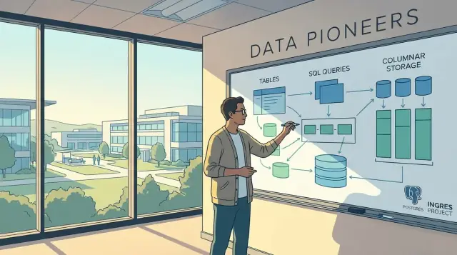
Why Stonebraker’s Work Still Shows Up in Your Data Stack

Michael Stonebraker is a computer scientist whose projects didn’t just influence database research—they directly shaped the products and design patterns many teams rely on every day. If you’ve used a relational database, an analytics warehouse, or a streaming system, you’ve benefited from ideas he helped prove, build, or popularize.

What you’ll get from this article

This isn’t a biography or an academic tour of database theory. Instead, it connects Stonebraker’s major systems (like Ingres, Postgres, and Vertica) to the choices you see in modern data stacks:

• Why SQL became the common language for data work
• Why analytics engines look and behave differently from OLTP databases
• Why “one database for everything” often fails in practice
• How architecture choices affect cost, performance, and reliability

What “modern database” means (plain English)

A modern database is any system that can reliably:

• Store data safely (so you don’t lose it)
• Query it quickly (so teams can answer questions)
• Scale as volume and users grow (without falling over)
• Stay correct under concurrency (so results match reality)

Different databases optimize these goals differently—especially when you compare transactional apps, BI dashboards, and real-time pipelines.

The promise of this piece

We’ll focus on practical impact: the ideas that show up in today’s “warehouse + lake + stream + microservices” world, and how they influence what you buy, build, and operate. Expect clear explanations, trade-offs, and real-world implications—not a deep dive into proofs or implementation details.

A Short, Useful Timeline of His Major Database Milestones

Stonebraker’s career is easiest to understand as a sequence of systems built for specific jobs—and then watched as the best ideas migrated into mainstream database products.

1970s: Ingres — making relational databases usable

Ingres began as an academic project that proved relational databases could be fast and practical, not just a theory. It helped popularize SQL-style querying and cost-based optimization thinking that later became normal in commercial engines.

1980s–1990s: Postgres — extensibility and “let the database evolve”

Postgres (the research system that led to PostgreSQL) explored a different bet: databases shouldn’t be fixed-function. You should be able to add new data types, new indexing methods, and richer behavior without rewriting the whole engine.

Many “modern” features trace back to this era—extensible types, user-defined functions, and a database that can adapt as workloads change.

2000s: Column stores and analytics-first design

As analytics grew, row-oriented systems struggled with large scans and aggregations. Stonebraker pushed columnar storage and related execution techniques aimed at reading only the columns you need and compressing them well—ideas that are now standard in analytics databases and cloud warehouses.

Mid-2000s: Vertica — MPP analytics as a product

Vertica took column-store research ideas into a commercially viable massively parallel processing (MPP) SQL engine designed for big analytic queries. This pattern repeats across the industry: a research prototype validates a concept; a product hardens it for reliability, tooling, and real customer constraints.

2010s and beyond: streaming and “right tool for the workload”

Later work expanded into stream processing and workload-specific engines—arguing that one general-purpose database rarely wins everywhere.

Research prototypes vs. products (why the distinction matters)

A prototype is built to test a hypothesis quickly; a product must prioritize operability: upgrades, monitoring, security, predictable performance, and support. Stonebraker’s influence shows up because many prototype ideas graduated into commercial databases as default capabilities rather than niche options.

Ingres: Making Relational Databases Practical

Ingres (short for INteractive Graphics REtrieval System) was Stonebraker’s early proof that the relational model could be more than an elegant theory. At the time, many systems were built around custom access methods and application-specific data paths.

Ingres set out to solve a simple, business-friendly problem:

How do you let people ask flexible questions of data without rewriting the software every time the question changes?

What Ingres was trying to fix

Relational databases promised you could describe what you want (e.g., “customers in California with overdue invoices”) rather than how to fetch it step by step. But making that promise real required a system that could:

• Store data reliably in tables
• Accept a high-level query language close to SQL
• Turn that query into an efficient plan automatically

Ingres was a major step toward that “practical” version of relational computing—one that could run on the hardware of the day and still feel responsive.

SQL adoption and the birth of query optimization basics

Ingres helped popularize the idea that a database should do the hard work of planning queries. Instead of developers hand-tuning every data access path, the system could choose strategies like which table to read first, which indexes to use, and how to join tables.

This helped SQL-style thinking spread: when you can write declarative queries, you can iterate faster, and more people can ask questions directly—analysts, product teams, even finance—without waiting for bespoke reports.

Why cost-based optimization matters

The big practical insight is cost-based optimization: pick the query plan with the lowest expected “cost” (usually a mix of I/O, CPU, and memory), based on statistics about the data.

That matters because it often means:

• Faster queries with no change to the application
• Less hardware needed to hit the same performance target
• More predictable performance as datasets grow

Ingres didn’t invent every piece of modern optimization, but it helped establish the pattern: SQL + an optimizer is what makes relational systems scale from “nice idea” to daily tool.

Postgres: The Big Idea of Extensible Databases

Early relational databases tended to assume a fixed set of data types (numbers, text, dates) and a fixed set of operations (filter, join, aggregate). That worked well—until teams started storing new kinds of information (geography, logs, time series, domain-specific identifiers) or needed specialized performance features.

With a rigid design, every new requirement turns into a bad choice: force-fit the data into text blobs, bolt on a separate system, or wait for a vendor to add support.

Extensibility, explained without the jargon

Postgres pushed a different idea: a database should be extensible—meaning you can add new capabilities in a controlled way, without breaking the safety and correctness you expect from SQL.

In plain language, extensibility is like adding certified attachments to a power tool rather than rewiring the motor yourself. You can teach the database “new tricks,” while still keeping transactions, permissions, and query optimization working as a coherent whole.

How this shaped modern extension ecosystems

That mindset shows up clearly in today’s PostgreSQL ecosystem (and many Postgres-inspired systems). Instead of waiting for a core feature, teams can adopt vetted extensions that integrate cleanly with SQL and operational tooling.

Common high-level examples include:

• Custom data types: store richer values (for example, geospatial points, ranges, or JSON-like structures) as first-class citizens.
• Custom functions: add domain logic that can be used directly in queries and reports.
• Indexing options: choose different index types for different access patterns, so the same SQL query can run much faster.

The key is that Postgres treated “changing what the database can do” as a design goal—not an afterthought—and that idea still influences how modern data platforms evolve.

Transactions and Concurrency: Getting Correct Results at Scale

Databases aren’t just about storing information—they’re about making sure the information stays right, even when many things happen at once. That’s what transactions and concurrency control are for, and it’s a major reason SQL systems became trusted for real business work.

What a transaction really guarantees

A transaction is a group of changes that must succeed or fail as a unit.

If you transfer money between accounts, place an order, or update inventory, you can’t afford “half-finished” results. A transaction ensures you don’t end up with an order that charged a customer but didn’t reserve stock—or stock that was reduced without an order being recorded.

In practical terms, transactions give you:

• Consistency you can explain to humans: the database doesn’t “kind of” apply changes.
• Recoverability: if something crashes mid-update, the system can roll back to a safe state.

Concurrency: the real-world mess databases must handle

Concurrency means many people (and apps) reading and changing data at the same time: customer checkouts, support agents editing accounts, background jobs updating statuses, analysts running reports.

Without careful rules, concurrency creates problems like:

• Lost updates: two users edit the same record; one overwrites the other.
• Dirty reads: someone sees data that later gets rolled back.
• Inconsistent reports: a query sees a mix of “before” and “after” states.

MVCC in plain language

One influential approach is MVCC (Multi-Version Concurrency Control). Conceptually, MVCC keeps multiple versions of a row for a short time, so readers can keep reading a stable snapshot while writers are making updates.

The big benefit is that reads don’t block writes as often, and writers don’t constantly stall behind long-running queries. You still get correctness, but with less waiting.

Why this matters in modern SQL workloads

Today’s databases often serve mixed workloads: high-volume app writes plus frequent reads for dashboards, customer views, and operational analytics. Modern SQL systems lean on techniques like MVCC, smarter locking, and isolation levels to balance speed with correctness—so you can scale activity without trading away trust in the data.

Column Stores: A Turning Point for Analytics Performance

Row-oriented databases were built for transaction processing: lots of small reads and writes, typically touching one customer, one order, one account at a time. That design is great when you need to fetch or update an entire record quickly.

Rows vs. columns (an everyday analogy)

Think of a spreadsheet. A row store is like filing each row as its own folder: when you need “everything about Order #123,” you pull one folder and you’re done. A column store is like filing by column: one drawer for “order_total,” another for “order_date,” another for “customer_region.”

For analytics, you rarely need the whole folder—you’re usually asking questions like “What was total revenue by region last quarter?” That query might touch only a few fields across millions of records.

Why analytics workloads love columns

Analytics queries often:

• Scan large portions of a table
• Use only a handful of columns
• Aggregate (SUM/AVG/COUNT) and filter heavily

With columnar storage, the engine can read only the columns referenced in the query, skipping the rest. Less data read from disk (and less moved through memory) is often the biggest performance win.

Compression isn’t just about saving space

Columns tend to have repetitive values (regions, statuses, categories). That makes them highly compressible—and compression can speed analytics because the system reads fewer bytes and can sometimes operate on compressed data more efficiently.

The bigger shift

Column stores helped mark the move from OLTP-first databases toward analytics-first engines, where scanning, compression, and fast aggregates became primary design goals rather than afterthoughts.

Vertica and MPP Analytics: Scaling SQL for Big Queries

Vertica is one of the clearest “real-world” examples of how Stonebraker’s ideas about analytics databases turned into a product teams could run in production. It took lessons from columnar storage and paired them with a distributed design aimed at a specific problem: answering big analytical SQL queries fast, even when data volumes grow beyond a single server.

What MPP means (in plain English)

MPP stands for massively parallel processing. The simplest way to think about it is: many machines work on one SQL query at the same time.

Instead of one database server reading all the data and doing all the grouping and sorting, the data is split across nodes. Each node processes its slice in parallel, and the system combines the partial results into a final answer.

This is how a query that would take minutes on one box can drop to seconds when spread across a cluster—assuming the data is distributed well and the query can be parallelized.

What it enables in practice

Vertica-style MPP analytics systems shine when you have lots of rows and want to scan, filter, and aggregate them efficiently. Typical use cases include:

• Dashboards that read large fact tables (product analytics, marketing performance, operational metrics)
• Scheduled reporting and ad-hoc “slice and dice” analysis in SQL
• Large aggregations (daily cohorts, funnels, top-N queries, rollups by many dimensions)

The trade-offs vs transactional databases

MPP analytics engines are not a drop-in replacement for transactional (OLTP) systems. They’re optimized for reading many rows and computing summaries, not for handling lots of small updates.

That leads to common trade-offs:

• Freshness: data often arrives in batches or micro-batches rather than row-by-row
• Updates: frequent single-row updates/deletes are typically slower or more operationally complex
• Latency: great for seconds-to-minutes analytical queries; not ideal for millisecond user-facing transactions

The key idea is focus: Vertica and similar systems earn their speed by tuning storage, compression, and parallel execution for analytics—then accepting constraints that transactional systems are designed to avoid.

Query Execution Innovations That Made Analytics Faster

A database can “store and query” data and still feel slow for analytics. The difference is often not the SQL you write, but how the engine executes it: how it reads pages, moves data through the CPU, uses memory, and minimizes wasted work.

Stonebraker’s analytics-focused projects pushed the idea that query performance is an execution problem as much as a storage problem. This thinking helped shift teams from optimizing single-row lookups to optimizing long scans, joins, and aggregations over millions (or billions) of rows.

Vectorized execution (work in batches, not one row at a time)

Many older engines process queries “tuple-at-a-time” (row-by-row), which creates lots of function calls and overhead. Vectorized execution flips that model: the engine processes a batch (a vector) of values in a tight loop.

In plain terms, it’s like moving groceries with a cart instead of carrying one item per trip. Batching reduces overhead and lets modern CPUs do what they’re good at: predictable loops, fewer branches, and better cache use.

Memory-friendly analytics design

Fast analytics engines are obsessed with staying CPU- and cache-efficient. Execution innovations commonly focus on:

• Avoiding unnecessary materialization (don’t build big intermediate tables if you can stream results forward)
• Working on compressed data where possible (less memory bandwidth, fewer bytes moved)
• Keeping hot data in cache (layout and batching that match how CPUs actually access memory)

These ideas matter because analytics queries are often limited by memory bandwidth and cache misses, not by raw disk speed.

Where you see this today

Modern data warehouses and SQL engines—cloud warehouses, MPP systems, and fast in-process analytics tools—frequently use vectorized execution, compression-aware operators, and cache-friendly pipelines as standard practice.

Even when vendors market features like “autoscaling” or “separation of storage and compute,” the day-to-day speed you feel still depends heavily on these execution choices.

If you’re evaluating platforms, ask not only what they store, but how they run joins and aggregates under the hood—and whether their execution model is built for analytics rather than transactional workloads.

Streaming Systems: From Batch Thinking to Real-Time Data

Streaming data is simply data that arrives continuously as a sequence of events—think “a new thing just happened” messages. A credit-card swipe, a sensor reading, a click on a product page, a package scan, a log line: each one shows up in real time and keeps coming.

Why batch databases feel slow for live work

Traditional databases and batch pipelines are great when you can wait: load yesterday’s data, run reports, publish dashboards. But real-time needs don’t wait for the next hourly job.

If you only process data in batches, you often end up with:

• Stale metrics (the numbers lag behind what’s happening)
• Delayed alerts (you find out after damage is done)
• Awkward workarounds (polling tables, constantly re-running queries)

Streaming systems are designed around the idea that computations can run continuously as events arrive.

The core ideas: continuous queries and windows

A continuous query is like a SQL query that never “finishes.” Instead of returning a result once, it updates the result as new events come in.

Because streams are unbounded (they don’t end), streaming systems use windows to make calculations manageable. A window is a slice of time or events, such as “the last 5 minutes,” “each minute,” or “the last 1,000 events.” This lets you compute rolling counts, averages, or top-N lists without needing to reprocess everything.

Business examples that benefit immediately

Real-time streaming is most valuable when timing matters:

• Fraud monitoring: flag unusual spending within seconds
• Operational alerts: detect error spikes or failing services as they start
• Live product metrics: see signups, conversions, or inventory changes as they happen
• Logistics visibility: update estimated delivery times from continuous scans

Workload-Driven Architecture: Using the Right Engine for the Job

Stonebraker has argued for decades that databases shouldn’t all be built as general-purpose “do everything” machines. The reason is simple: different workloads reward different design choices. If you optimize hard for one job (say, tiny transactional updates), you usually make another job slower (like scanning billions of rows for a report).

Why teams end up with multiple systems

Most modern stacks use more than one data system because the business asks for more than one kind of answer:

• OLTP database (app database): fast inserts/updates, strict correctness, many concurrent users
• Warehouse / analytics database: fast reads over lots of data, heavy aggregations, long scans
• Cache / key-value store: extremely fast reads for “hot” data (sessions, counters, feature flags)
• Stream processing + log: handles continuous events (clicks, payments, IoT), low-latency pipelines, real-time metrics

That’s “one size doesn’t fit all” in practice: you pick engines that match the shape of the work.

A simple decision guide

Use this quick filter when choosing (or justifying) another system:

• If you need many small reads/writes with transactions (orders, user profiles): start with an OLTP DB.
• If you need big queries and aggregates (weekly revenue, cohort analysis): add an analytics warehouse.
• If you need sub-second responses on repeated lookups: introduce a cache.
• If you need real-time reactions to events (fraud rules, live dashboards): add streaming.

Avoid tool sprawl

Multiple engines can be healthy, but only when each one has a clear workload. A new tool should earn its place by cutting cost, latency, or risk—not by adding novelty.

Prefer fewer systems with strong operational ownership, and retire components that don’t have a crisp, measurable purpose.

How These Ideas Show Up in Modern Data Architecture

Stonebraker’s research threads—relational foundations, extensibility, column stores, MPP execution, and “right tool for the job”—are visible in the default shapes of modern data platforms.

Familiar architecture patterns (and why they look this way)

The warehouse reflects decades of work on SQL optimization, columnar storage, and parallel execution. When you see fast dashboards on huge tables, you’re often seeing column-oriented formats plus vectorized processing and MPP-style scaling.

The lakehouse borrows warehouse ideas (schemas, statistics, caching, cost-based optimization) but places them on open file formats and object storage. The “storage is cheap, compute is elastic” shift is new; the query and transaction thinking underneath is not.

MPP analytics systems (shared-nothing clusters) are direct descendants of research that proved you can scale SQL by partitioning data, moving computation to data, and carefully managing data movement during joins and aggregations.

Where SQL fits today

SQL has become the common interface across warehouses, MPP engines, and even “lake” query layers. Teams rely on it as:

• A stable contract for BI tools and analysts
• A portability layer when engines change
• A governance surface (views, permissions, audited access)

Even when execution happens in different engines (batch, interactive, streaming), SQL often remains the user-facing language.

Data modeling and governance: schemas still matter

Flexible storage doesn’t eliminate the need for structure. Clear schemas, documented meaning, and controlled evolution reduce downstream breakage.

Good governance is less about bureaucracy and more about making data reliable: consistent definitions, ownership, quality checks, and access controls.

A no-hype checklist for choosing an approach

When evaluating platforms, ask:

1. Workload fit: Is it mainly BI dashboards, ad-hoc exploration, ML feature building, or operational workloads?
2. Latency needs: Seconds, minutes, or hours? Do you need streaming freshness?
3. Data shape: Mostly wide event logs (great for columnar) or many point lookups (often better elsewhere)?
4. Concurrency: How many users/queries at once, and how predictable are they?
5. Consistency requirements: Do you need strong transactions, or is eventual consistency acceptable?
6. Operational reality: Who will run it, what skills exist, and what’s the failure mode at 2 a.m.?

If a vendor can’t map their product to these basics in plain language, the “innovation” might be mostly packaging.

Key Takeaways for Teams Building or Buying Data Platforms

Stonebraker’s through-line is simple: databases work best when they’re designed for a specific job—and when they can evolve as that job changes.

1) Match the system to the workload (don’t expect one engine to win everywhere)

Before comparing features, write down what you actually need to do:

• Analytics: long scans, big aggregations, lots of reads
• Transactions: many small updates, strict correctness, fast response times
• Mixed workloads: both, but often at the cost of careful tuning and clear priorities
• Real-time feeds: continuous ingestion and incremental computation

A useful rule: if you can’t describe your workload in a few sentences (query patterns, data size, latency needs, concurrency), you’ll end up shopping by buzzwords.

2) Design for change, not just for today’s schema

Teams underestimate how often requirements shift: new data types, new metrics, new compliance rules, new consumers.

Favor platforms and data models that make change routine rather than risky:

• Clear separation between storage, querying, and extension points
• Safe ways to evolve schemas and roll out new logic
• Measurable performance that doesn’t collapse with organic growth

3) Correctness is a product feature

Fast answers are only valuable if they’re the right answers. When evaluating options, ask how the system handles:

• Concurrent writes (what happens when two people/processes update the same record?)
• Isolation and consistency (what guarantees do you get, and what do you trade to get them?)
• Operational failure modes (restarts, partial outages, backfills)

4) Practical evaluation checklist for non-specialists

Run a small “proof with your data,” not just a demo:

• Try 3–5 representative queries and measure time and cost.
• Test peak concurrency (the Monday-morning spike).
• Validate data freshness, recovery steps, and who can operate it day-to-day.

5) Turning architecture decisions into shipping software

A lot of database guidance stops at “pick the right engine,” but teams also have to ship apps and internal tools around that engine: admin panels, metrics dashboards, ingestion services, and back-office workflows.

If you want to prototype these quickly without reinventing your whole pipeline, a vibe-coding platform like Koder.ai can help you spin up web apps (React), backend services (Go + PostgreSQL), and even mobile clients (Flutter) from a chat-driven workflow. That’s often useful when you’re iterating on schema design, building a small internal “data product,” or validating how a workload actually behaves before committing to long-term infrastructure.

Next reading (to build intuition)

If you want to go deeper, look up columnar storage, MVCC, MPP execution, and stream processing. More explainers live in /blog.