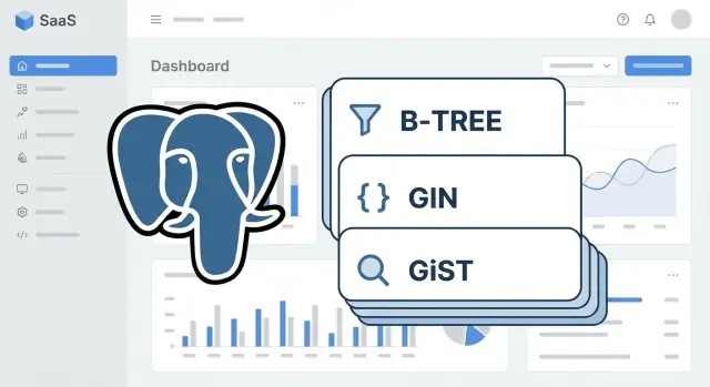
PostgreSQL indexes for SaaS apps: btree vs GIN vs GiST

What problem indexes solve in real SaaS screens

An index changes how PostgreSQL finds rows. Without an index, the database often has to read a lot of the table (a sequential scan) and then discard most of it. With the right index, it can jump straight to the matching rows (an index lookup), then fetch only what it needs.

You notice this early in SaaS because everyday screens are query-heavy. A single click can trigger several reads: the list page, a total count, a couple of dashboard cards, and a search box. When a table grows from thousands to millions of rows, the same query that used to feel instant starts to lag.

A typical example is an Orders page filtered by status and date, sorted by newest first, with pagination. If PostgreSQL has to scan the whole orders table to find paid orders from the last 30 days, every page load does extra work. A good index turns that into a quick hop to the right slice of data.

Indexes aren’t free. Each one buys faster reads for specific queries, but it also makes writes slower (INSERT/UPDATE/DELETE must update indexes) and uses more storage (plus more cache pressure). That trade-off is why you should start from real query patterns, not from index types.

A simple rule that prevents busywork: add an index only when you can point to a specific, frequent query it will speed up. If you build screens with a chat-driven builder like Koder.ai, it helps to capture the SQL behind your list pages and dashboards and use that as your index wish list.

B-tree vs GIN vs GiST in plain terms

Most indexing confusion goes away when you stop thinking in features (JSON, search, arrays) and start thinking in query shape: what does the WHERE clause do, and how do you expect results to be ordered?

B-tree: fast for ordering and comparisons

Use B-tree when your query looks like normal comparisons and you care about sort order. It’s the workhorse for equality, ranges, and joins.

Example shapes: filtering by tenant_id = ?, status = 'active', created_at >= ?, joining users.id = orders.user_id, or showing “latest first” with ORDER BY created_at DESC.

GIN and GiST: when a row contains many searchable values

GIN (Generalized Inverted Index) is a good fit when one column contains many members and you ask, “does it contain X?” That’s common with JSONB keys, array elements, and full-text vectors.

Example shapes: metadata @> {'plan':'pro'} on JSONB, tags @> ARRAY['urgent'], or to_tsvector(body) @@ plainto_tsquery('reset password').

GiST (Generalized Search Tree) fits questions about distance or overlap, where values behave like ranges or shapes. It’s often used for range types, geometric data, and some “closest match” searches.

Example shapes: overlapping time windows with range columns, some similarity-style searches (for example, with trigram operators), or spatial queries (if you use PostGIS).

A practical way to choose:

• If you filter or sort by normal columns, start with B-tree.
• If you check containment or membership, look at GIN.
• If you ask “how close” or “does it overlap,” GiST is often the fit.
• If a query is rare or a table is tiny, you might not need a new index.
• If you can’t describe the query shape, measure first (EXPLAIN) before adding anything.

Indexes speed reads, but they cost write time and disk. In SaaS, that trade-off matters most on hot tables like events, sessions, and activity logs.

B-tree patterns for filters, sorting, and pagination

Most SaaS list screens share the same shape: a tenant boundary, a couple of filters, and a predictable sort. B-tree indexes are the default choice here, and they’re usually the cheapest to maintain.

A common pattern is WHERE tenant_id = ? plus filters like status = ?, user_id = ?, and a time range like created_at >= ?. For composite B-tree indexes, put equality filters first (columns you match with =), then add the column you sort by.

Rules that work well in most apps:

• Start with tenant_id if every query is tenant-scoped.
• Put = filters next (often status, user_id).
• Put the ORDER BY column last (often created_at or id).
• Use INCLUDE to cover list pages without making the key wider.
• Prefer seek pagination over offset when pages get deep.

A realistic example: a Tickets page showing the newest items first, filtered by status.

-- Query
SELECT id, status, created_at, title
FROM tickets
WHERE tenant_id = $1
  AND status = $2
ORDER BY created_at DESC
LIMIT 50;

-- Index
CREATE INDEX tickets_tenant_status_created_at_idx
ON tickets (tenant_id, status, created_at DESC)
INCLUDE (title);

That index supports both the filter and the sort, so Postgres can avoid sorting a large result set. The INCLUDE (title) part helps the list page touch fewer table pages, while keeping the index keys focused on filtering and ordering.

For time ranges, the same idea applies:

SELECT id, created_at
FROM events
WHERE tenant_id = $1
  AND created_at >= $2
  AND created_at <  $3
ORDER BY created_at DESC
LIMIT 100;

CREATE INDEX events_tenant_created_at_idx
ON events (tenant_id, created_at DESC);

Pagination is where many SaaS apps slow down. Offset pagination (OFFSET 50000) forces the database to walk past many rows. Seek pagination stays fast by using the last seen sort key:

SELECT id, created_at
FROM tickets
WHERE tenant_id = $1
  AND created_at < $2
ORDER BY created_at DESC
LIMIT 50;

With the right B-tree index, this stays quick even as the table grows.

Tenant-friendly indexing without over-indexing

Most SaaS apps are multi-tenant: every query must stay inside one tenant. If your indexes don’t include tenant_id, Postgres can still find rows quickly, but it often scans far more index entries than needed. Tenant-aware indexes keep each tenant’s data clustered in the index so common screens stay fast and predictable.

A simple rule: put tenant_id first in the index when the query always filters by tenant. Then add the column you filter or sort by most.

High-impact, boring indexes often look like:

• (tenant_id, created_at) for recent-items lists and cursor pagination
• (tenant_id, status) for status filters (Open, Paid, Failed)
• (tenant_id, user_id) for “items owned by this user” screens
• (tenant_id, updated_at) for “recently changed” admin views
• (tenant_id, external_id) for lookups from webhooks or imports

Over-indexing happens when you add a new index for every slightly different screen. Before creating another one, check if an existing composite index already covers the leftmost columns you need. For example, if you have (tenant_id, created_at), you usually don’t also need (tenant_id, created_at, id) unless you truly filter on id after those columns.

Partial indexes can cut size and write cost when most rows aren’t relevant. They work well with soft deletes and “active only” data, for example: index only where deleted_at IS NULL, or only where status = 'active'.

Every extra index makes writes heavier. Inserts must update each index, and updates can touch multiple indexes even when you change one column. If your app ingests lots of events (including apps built quickly with Koder.ai), keep indexes focused on the few query shapes users hit every day.

Indexing JSONB: GIN and targeted expression indexes

JSONB is handy when your app needs flexible extra fields like feature flags, user attributes, or per-tenant settings. The catch is that different JSONB operators behave differently, so the best index depends on how you query.

Two shapes matter most:

• Containment: “Does this JSON contain these key-value pairs?” using @>.
• Path extraction: “What is the value of this specific field?” using -> / ->> (often compared with =).

When a GIN index is the right fit

If you frequently filter with @>, a GIN index on the JSONB column usually pays off.

-- Query shape: containment
SELECT id
FROM accounts
WHERE tenant_id = $1
  AND metadata @> '{"region":"eu","plan":"pro"}';

-- Index
CREATE INDEX accounts_metadata_gin
ON accounts
USING GIN (metadata);

If your JSON structure is predictable and you mostly use @> on top-level keys, jsonb_path_ops can be smaller and faster, but it supports fewer operator types.

When an expression index is better

If your UI repeatedly filters on one field (like plan), extracting that field and indexing it is often faster and cheaper than a wide GIN.

SELECT id
FROM accounts
WHERE tenant_id = $1
  AND metadata->>'plan' = 'pro';

CREATE INDEX accounts_plan_expr
ON accounts ((metadata->>'plan'));

A practical rule: keep JSONB for flexible, rarely filtered attributes, but promote stable, high-usage fields (plan, status, created_at) into real columns. If you’re iterating fast on a generated app, it’s often an easy schema tweak once you see which filters show up on every page.

Example: if you store {"tags":["beta","finance"],"region":"us"} in JSONB, use GIN when you filter by bundles of attributes (@>), and add expression indexes for the few keys that drive most list views (plan, region).

Indexing arrays: when GIN shines

Arrays look tempting because they’re easy to store and easy to read. A users.roles text[] column or projects.labels text[] column can work well when you mostly ask one question: does this row contain a value (or a set of values)? That’s exactly where a GIN index helps.

GIN is the go-to choice for membership queries on arrays. It breaks the array into individual items and builds a fast lookup to rows that contain them.

Array query shapes that often benefit:

• Contains a value or set: @> (array contains)
• Overlap with a set: && (array shares any items)
• Sometimes: = ANY(...), but @> is often more predictable

A typical example for filtering users by role:

-- Find users who have the "admin" role
SELECT id, email
FROM users
WHERE roles @> ARRAY['admin'];

CREATE INDEX users_roles_gin ON users USING GIN (roles);

And filtering projects by a label set (must include both labels):

SELECT id, name
FROM projects
WHERE labels @> ARRAY['billing', 'urgent'];

CREATE INDEX projects_labels_gin ON projects USING GIN (labels);

Where people get surprised: some patterns don’t use the index the way you expect. If you turn the array into a string (array_to_string(labels, ',')) and then run LIKE, the GIN index won’t help. Also, if you need “starts with” or fuzzy matches inside labels, you’re in text search territory, not array membership.

Arrays can also become hard to maintain when they turn into a mini-database: frequent updates, needing metadata per item (who added the label, when, why), or needing analytics per label. At that point, a join table like project_labels(project_id, label) is usually easier to validate, query, and evolve.

Search indexing: full-text and fuzzy matching (GIN and GiST)

For search boxes, two patterns show up again and again: full-text search (find records about a topic) and fuzzy matching (handle typos, partial names, and ILIKE patterns). The right index is the difference between “instant” and “timeouts at 10k users”.

Full-text search: tsvector + GIN

Use full-text search when users type real words and you want results ranked by relevance, like searching tickets by subject and description. The usual setup is to store a tsvector (often in a generated column) and index it with GIN. You search with @@ and a tsquery.

-- Tickets: full-text search on subject + body
ALTER TABLE tickets
ADD COLUMN search_vec tsvector
GENERATED ALWAYS AS (
  to_tsvector('simple', coalesce(subject,'') || ' ' || coalesce(body,''))
) STORED;

CREATE INDEX tickets_search_vec_gin
ON tickets USING GIN (search_vec);

-- Query
SELECT id, subject
FROM tickets
WHERE search_vec @@ plainto_tsquery('simple', 'invoice failed');

-- Customers: fuzzy name search using trigrams
CREATE INDEX customers_name_trgm
ON customers USING GIN (name gin_trgm_ops);

SELECT id, name
FROM customers
WHERE name ILIKE '%jon smth%';

What to store in the vector: only the fields you actually search. If you include everything (notes, internal logs), you pay in index size and write cost.

Fuzzy matching: trigrams with GIN or GiST

Use trigram similarity when users search names, emails, or short phrases and you need partial matches or typo tolerance. Trigrams help with ILIKE '%term%' and similarity operators. GIN is usually faster for “does it match?” lookups; GiST can be a better fit when you also care about ordering by similarity.

Rules of thumb:

• Use GIN + tsvector for relevance-based text search.
• Use trigrams for ILIKE and typo-friendly name searches.

Pitfalls worth watching:

• Leading wildcards without trigrams (ILIKE '%abc') force scans.
• Very short search terms (1-2 chars) often can’t use trigrams well.
• Stop words and stemming can surprise users in full-text results, so pick a configuration that matches your product language.

If you’re shipping search screens quickly, treat the index as part of the feature: search UX and index choice need to be designed together.

Step by step: from slow query to the right index

Start with the exact query your app runs, not a guess. A “slow screen” is usually one SQL statement with a very specific WHERE and ORDER BY. Copy it from logs, your ORM debug output, or whatever query capture you already use.

A workflow that holds up in real apps:

• Capture the full SQL, including WHERE, ORDER BY, and LIMIT.
• Run EXPLAIN (ANALYZE, BUFFERS) on the same query.
• Focus on the operators doing the work (=, >=, LIKE, @>, @@), not just the column names.
• Add the smallest index that matches those operators.
• Re-run EXPLAIN (ANALYZE, BUFFERS) with realistic data volume.

Here’s a concrete example. A Customers page filters by tenant and status, sorts by newest, and paginates:

SELECT id, created_at, email
FROM customers
WHERE tenant_id = $1 AND status = $2
ORDER BY created_at DESC
LIMIT 50;

If EXPLAIN shows a sequential scan and a sort, a B-tree index that matches the filter and sort often fixes it:

CREATE INDEX ON customers (tenant_id, status, created_at DESC);

If the slow part is JSONB filtering like metadata @> '{"plan":"pro"}', that points to GIN. If it’s full-text search like to_tsvector(...) @@ plainto_tsquery(...), that also points to a GIN-backed search index. If it’s a “closest match” or overlap-style operator set, that’s where GiST is often the fit.

After adding the index, measure the trade-off. Check index size, insert and update time, and whether it helps the top few slow queries or only one edge case. In fast-moving projects (including ones built on Koder.ai), this re-check helps you avoid piling up unused indexes.

Common indexing mistakes that waste time and money

Most index problems aren’t about choosing B-tree vs GIN vs GiST. They’re about building an index that looks right, but doesn’t match how the app queries the table.

Mistakes that tend to hurt most:

• Indexes that never get used. The query uses a different operator than the index supports, or a composite index has the wrong column order. If your WHERE clause starts with tenant_id and created_at, but the index starts with created_at, the planner may skip it.
• Indexing low-cardinality columns alone. A lone index on status, is_active, or a boolean often does little because it matches too many rows. Pair it with a selective column (like tenant_id or created_at) or skip it.
• Overlapping indexes that bloat and slow writes. Similar indexes on the same table can double storage and make inserts and updates slower.
• Pagination blind spots. Indexing only to support OFFSET is a common trap. If you use keyset pagination, you need an index that matches the sort and the last-seen filter.
• Stale stats and table clutter. If autovacuum isn’t keeping up, or ANALYZE hasn’t run recently, the planner can choose bad plans even when the right index exists.

A concrete example: your Invoices screen filters by tenant_id and status, then sorts by created_at DESC. An index on just status will barely help. A better fit is a composite index that starts with tenant_id, then status, then created_at (filter first, sort last). That single change often beats adding three separate indexes.

Treat every index as a cost. It has to earn its keep in real queries, not just in theory.

Quick checklist before shipping index changes

Index changes are easy to ship and annoying to undo if they add write cost or lock a busy table. Before you merge, treat it like a small release.

Start by deciding what you’re optimizing. Pull two short rankings from your logs or monitoring: the queries that run most often, and the queries with the highest latency. For each, write down the exact shape: filter columns, sort order, joins, and operators used (equals, range, IN, ILIKE, JSONB operators, array contains). This prevents guessing and helps you pick the right index type.

Pre-ship checklist:

• Confirm the query is tenant-scoped where it should be.
• Match the index to the operator: B-tree for equality/range/sort, GIN for membership (arrays, JSONB, full text), GiST for specialty overlap or distance-style cases.
• Prefer one composite index that matches the common filter + sort, instead of several single-column indexes.
• Keep the index narrow: only include columns the query truly uses.
• Plan the rollout: will index creation block writes, and do you need to schedule it off-peak?

After you add the index, verify it helped in the real plan. Run EXPLAIN (ANALYZE, BUFFERS) on the exact query and compare before vs after. Then watch production behavior for a day:

• Did read latency drop for the target screens?
• Did write latency increase (inserts/updates)?
• Did CPU or storage spike due to the new index?
• Is the index actually used, or is it dead weight?

If you’re building with Koder.ai, it’s worth keeping the generated SQL for one or two slow screens next to the change, so the index matches what the app actually runs.

Example: indexing a typical SaaS app workflow + next steps

Picture a common admin screen: a Users list with tenant scoping, a few filters, sort by last active, and a search box. This is where indexes stop being theory and start saving real time.

Three query shapes you’ll usually see:

-- 1) List page with tenant + status filter + sort
SELECT id, email, last_active_at
FROM users
WHERE tenant_id = $1 AND status = $2
ORDER BY last_active_at DESC
LIMIT 50;

-- 2) Search box (full-text)
SELECT id, email
FROM users
WHERE tenant_id = $1
  AND to_tsvector('simple', coalesce(name,'') || ' ' || coalesce(email,'')) @@ plainto_tsquery($2)
ORDER BY last_active_at DESC
LIMIT 50;

-- 3) Filter on JSON metadata (plan, flags)
SELECT id
FROM users
WHERE tenant_id = $1
  AND metadata @> '{"plan":"pro"}'::jsonb;

A small but intentional index set for this screen:

• B-tree composite for the list view: (tenant_id, status, last_active_at DESC).
• GIN for search: a generated tsvector column with a GIN index.
• JSONB indexing based on usage: GIN (metadata) when you use @> a lot, or an expression B-tree like ((metadata->>'plan')) when you mostly filter a single key.

Mixed needs are normal. If one page does filters + search + JSON, avoid cramming everything into one mega index. Keep the B-tree for sorting/pagination, then add one specialized index (often GIN) for the expensive part.

Next steps: pick one slow screen, write down its top 2-3 query shapes, and review each index by purpose (filter, sort, search, JSON). If an index doesn’t clearly match a real query, drop it from the plan. If you’re iterating quickly on koder.ai, doing this review as you add new screens can prevent index sprawl while your schema is still changing.