Why Time-Series Databases Matter for Metrics and Observability

Metrics, Monitoring, and Observability: The Basics

Metrics are numbers that describe what your system is doing—measurements you can chart, like request latency, error rate, CPU usage, queue depth, or active users.

Monitoring is the practice of collecting those measurements, putting them on dashboards, and setting alerts when something looks wrong. If a checkout service’s error rate spikes, monitoring should tell you quickly and clearly.

Observability goes a step further: it’s your ability to understand why something is happening by looking at multiple signals together—typically metrics, logs, and traces. Metrics tell you what changed, logs give you what happened, and traces show you where time was spent across services.

Why time-based data is different

Time-series data is “value + timestamp,” repeated constantly.

That time component changes how you use the data:

• You ask questions like “What’s the trend over the last 15 minutes?” or “Did this get worse after a deploy?”
• You care about recent data being fast to query for dashboards and alerts.
• You often aggregate (avg/p95/sum) across time windows rather than pulling individual rows.

What a TSDB solves (and what it doesn’t)

A time-series database (TSDB) is optimized to ingest lots of timestamped points, store them efficiently, and query them quickly over time ranges.

A TSDB won’t magically fix missing instrumentation, unclear SLOs, or noisy alerts. It also won’t replace logs and traces; it complements them by making metric workflows reliable and cost-effective.

Quick example: latency over time

Imagine you chart your API’s p95 latency every minute. At 10:05 it jumps from 180ms to 900ms and stays there. Monitoring raises an alert; observability helps you connect that spike to a specific region, endpoint, or deployment—starting from the metric trend and drilling into the underlying signals.

What Makes Time-Series Data Unique

Time-series metrics have a simple shape, but their volume and access patterns make them special. Each data point is typically timestamp + labels/tags + value—for example: “2025-12-25 10:04:00Z, service=checkout, instance=i-123, p95_latency_ms=240”. The timestamp anchors the event in time, labels describe which thing emitted it, and the value is what you want to measure.

A write pattern built for constant flow

Metrics systems don’t write in occasional batches. They write continuously, often every few seconds, from many sources at once. That creates a stream of lots of small writes: counters, gauges, histograms, and summaries arriving nonstop.

Even modest environments can produce millions of points per minute when you multiply scrape intervals by hosts, containers, endpoints, regions, and feature flags.

Reads are almost always “over a range”

Unlike transactional databases where you fetch “the latest row,” time-series users usually ask:

• “What happened over the last 15 minutes?”
• “Compare today vs. yesterday at the same time.”
• “Show p95/p99 latency by service for the last hour.”

That means common queries are range scans, rollups (e.g., 1s → 1m averages), and aggregations like percentiles, rates, and grouped sums.

The signals are in the shape of the line

Time-series data is valuable because it reveals patterns that are hard to spot in isolated events: spikes (incidents), seasonality (daily/weekly cycles), and long-term trends (capacity creep, gradual regressions). A database that understands time makes it easier to store these streams efficiently and query them fast enough for dashboards and alerting.

What a Time-Series Database (TSDB) Is

A time-series database (TSDB) is a database built specifically for time-ordered data—measurements that arrive continuously and are primarily queried by time. In monitoring, that usually means metrics like CPU usage, request latency, error rate, or queue depth, each recorded with a timestamp and a set of labels (service, region, instance, etc.).

Storage designed for time

Unlike general-purpose databases that store rows optimized for many access patterns, TSDBs optimize for the most common metrics workload: write new points as time moves forward and read recent history quickly. Data is typically organized in time-based chunks/blocks so the engine can scan “last 5 minutes” or “last 24 hours” efficiently without touching unrelated data.

Compression and encoding for numeric series

Metrics are often numeric and change gradually. TSDBs take advantage of that by using specialized encoding and compression techniques (for example, delta encoding between adjacent timestamps, run-length patterns, and compact storage for repeated label sets). The result: you can keep more history for the same storage budget, and queries read fewer bytes from disk.

Why append-only writes are fast

Monitoring data is mostly append-only: you rarely update old points; you add new ones. TSDBs lean into this pattern with sequential writes and batch ingestion. That reduces random I/O, lowers write amplification, and keeps ingestion stable even when many metrics arrive at once.

Common APIs and query styles

Most TSDBs expose query primitives tailored to monitoring and dashboards:

• Range queries: “give me this metric over the last N minutes.”
• Group by time: bucket data into intervals (e.g., 1m) for graphing and aggregation.
• Label filtering: select series by tags/labels (e.g., service="api", region="us-east").

Even when syntax differs across products, these patterns are the foundation for building dashboards and powering alert evaluations reliably.

Why TSDBs Fit Monitoring Workloads

Monitoring is a stream of small facts that never stops: CPU ticks every few seconds, request counts every minute, queue depth all day long. A TSDB is built for that pattern—continuous ingestion plus “what happened recently?” questions—so it tends to feel faster and more predictable than a general-purpose database when you use it for metrics.

Fast answers to time-based questions

Most operational questions are range queries: “show me the last 5 minutes,” “compare to the last 24 hours,” “what changed since deploy?” TSDB storage and indexing are optimized for scanning time ranges efficiently, which keeps charts snappy even as your dataset grows.

Aggregations that match how teams think

Dashboards and SRE monitoring rely on aggregations more than raw points. TSDBs typically make common metric math efficient:

• Averages over time windows (avg)
• Latency percentiles (p95/p99)
• Counter math like rate and increase

These operations are essential for turning noisy samples into signals you can alert on.

Time bucketing, rollups, and predictable costs

Dashboards rarely need every raw datapoint forever. TSDBs often support time bucketing and rollups, so you can store high-resolution data for recent periods and pre-aggregate older data for long-term trends. That keeps queries quick and helps control storage without losing the big picture.

Performance under constant ingestion

Metrics don’t arrive in batches; they arrive continuously. TSDBs are designed so write-heavy workloads don’t degrade read performance as quickly, helping ensure your “is something broken right now?” queries remain reliable during traffic spikes and incident storms.

High Cardinality: The Make-or-Break Factor for Metrics

Metrics become powerful when you can slice them by labels (also called tags or dimensions). A single metric like http_requests_total might be recorded with dimensions such as service, region, instance, and endpoint—so you can answer questions like “Is EU slower than US?” or “Is one instance misbehaving?”

What cardinality means (and why it explodes)

Cardinality is the number of unique time series your metrics create. Every unique combination of label values is a different series.

For example, if you track one metric with:

• 20 services
• 5 regions
• 200 instances
• 50 endpoints

…you already have 20 × 5 × 200 × 50 = 1,000,000 time series for that single metric. Add a few more labels (status code, method, user type) and it can grow beyond what your storage and query engine can handle.

What breaks first when cardinality is too high

High cardinality usually doesn’t fail gracefully. The first pain points tend to be:

• Memory pressure: the system needs to keep recent series and metadata “hot,” and memory usage climbs quickly.
• Index growth: the label index can become huge, increasing disk usage and slowing lookups.
• Query latency: dashboards and alert evaluations may scan or match far more series than intended, leading to slow panels and delayed alerts.

This is why high-cardinality tolerance is a key TSDB differentiator: some systems are designed to handle it; others get unstable or expensive fast.

Choosing labels: what to keep, what to avoid

A good rule: use labels that are bounded and low-to-medium variability, and avoid labels that are effectively unbounded.

Prefer:

• service, region, cluster, environment
• instance (if your fleet size is controlled)
• endpoint only if it’s a normalized route template (e.g., /users/:id, not /users/12345)

Avoid:

• User IDs, session IDs, request IDs, order IDs
• Full URLs with query strings
• Raw error messages or stack traces

If you need those details, keep them in logs or traces and link from a metric via a stable label. That way your TSDB stays fast, your dashboards stay usable, and your alerting stays on-time.

Retention, Downsampling, and Cost Control

Keeping metrics “forever” sounds appealing—until storage bills grow and queries slow down. A TSDB helps you keep the data you need, at the detail you need, for the time you need it.

Why compression matters

Metrics are naturally repetitive (same series, steady sampling interval, small changes between points). TSDBs take advantage of this with purpose-built compression, often storing long histories at a fraction of the raw size. That means you can retain more data for trend analysis—capacity planning, seasonal patterns, and “what changed since last quarter?”—without paying for equally large disks.

Retention: raw vs aggregated data

Retention is simply the rule for how long data is kept.

Most teams split retention into two layers:

• Raw (high-resolution) retention: keep per-second or per-10-second data for a shorter window (e.g., 7–30 days) to troubleshoot incidents with full detail.
• Aggregated retention: keep rolled-up data (e.g., 1-minute, 10-minute, 1-hour) for longer windows (e.g., 6–24 months) to track long-term behavior.

This approach prevents yesterday’s ultra-granular troubleshooting data from becoming next year’s expensive archive.

Downsampling / rollups: when to apply them

Downsampling (also called rollups) replaces many raw points with fewer summarized points—typically avg/min/max/count over a time bucket. Apply it when:

• You mostly need trends rather than point-by-point debugging.
• Dashboards cover weeks or months and don’t benefit from second-level detail.
• You want faster queries for wide time ranges.

Some teams downsample automatically after the raw window expires; others keep raw for “hot” services longer and downsample faster for noisy or low-value metrics.

The tradeoffs (precision, storage, speed)

Downsampling saves storage and speeds up long-range queries, but you lose detail. For example, a short CPU spike might disappear in a 1-hour average, while min/max rollups can preserve “something happened” without preserving exactly when or how often.

A practical rule: keep raw long enough to debug recent incidents, and keep rollups long enough to answer product and capacity questions.

Alerting Needs Reliable, Timely Queries

Alerts are only as good as the queries behind them. If your monitoring system can’t answer “is this service unhealthy right now?” quickly and consistently, you’ll either miss incidents or get paged for noise.

What alert queries look like

Most alert rules boil down to a few query patterns:

• Threshold checks: “CPU > 90% for 10 minutes,” or “error rate > 2%.”
• Rate and ratio checks: “5xx per second,” “errors / requests,” “queue depth increasing.” These often rely on functions like rate() over counters.
• Anomaly-style checks: “latency is unusually high compared to the last hour/day,” or “traffic dropped below expected.” These typically compare a current window to a baseline.

A TSDB matters here because these queries must scan recent data fast, apply aggregations correctly, and return results on schedule.

Evaluation windows: why timing matters

Alerts aren’t evaluated on single points; they’re evaluated over windows (for example, “last 5 minutes”). Small timing issues can change outcomes:

• Late ingestion can make a healthy system look broken (or hide a real outage).
• Misaligned windows can cause “almost always firing” rules when traffic is spiky.
• If queries are slow, your alerting loop drifts and decisions arrive too late.

Common pitfalls (and how to reduce them)

Noisy alerts often come from missing data, uneven sampling, or overly sensitive thresholds. Flapping—rapidly switching between firing and resolved—usually means the rule is too close to normal variance or the window is too short.

Treat “no data” explicitly (is it a problem, or just an idle service?), and prefer rate/ratio alerts over raw counts when traffic varies.

Make alerts actionable

Every alert should link to a dashboard and a short runbook: what to check first, what “good” looks like, and how to mitigate. Even a simple /runbooks/service-5xx and a dashboard link can cut response time dramatically.

Where TSDBs Fit in the Observability Stack

Observability usually combines three signal types: metrics, logs, and traces. A TSDB is the specialist store for metrics—data points indexed by time—because it’s optimized for fast aggregations, rollups, and “what changed in the last 5 minutes?” questions.

Metrics: fast detection and SLO tracking

Metrics are the best first line of defense. They’re compact, cheap to query at scale, and ideal for dashboards and alerting. This is how teams track SLOs like “99.9% of requests under 300ms” or “error rate below 1%.”

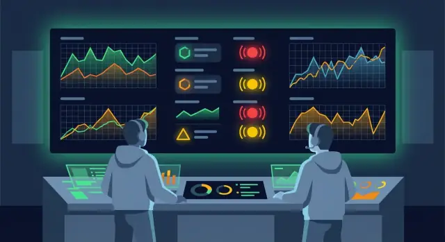
A TSDB typically powers:

• Real-time dashboards (service health, latency, saturation)
• Alert evaluations (thresholds, burn rates, anomaly-style checks)
• Historical reporting (weekly trends, capacity planning)

Logs and traces: context after you detect a problem

Metrics tell you that something is wrong, but not always why.

• Logs provide detailed event records (errors, warnings, business events). They answer “what happened?” and “which request failed?”
• Traces show end-to-end request paths across services. They answer “where did the time go?” and “which dependency caused the slowdown?”

A simple workflow: detect → triage → deep-dive

1. Detect (TSDB + alerts): an alert fires on elevated error rate or latency.
2. Triage (TSDB dashboards): narrow it down by service, region, version, or endpoint using metric dimensions.
3. Deep-dive (logs/traces): pivot to the correlated logs and traces for the specific time window to find the root cause.

In practice, a TSDB sits at the center of “fast signal” monitoring, while log and trace systems act as the high-detail evidence you consult once metrics show where to look.

Scalability and Reliability Considerations

Monitoring data is most valuable during an incident—exactly when systems are under stress and dashboards are getting hammered. A TSDB has to keep ingesting and answering queries even while parts of the infrastructure are degraded, otherwise you lose the timeline you need to diagnose and recover.

Scaling out: sharding and replication

Most TSDBs scale horizontally by sharding data across nodes (often by time ranges, metric name, or a hash of labels). This spreads write load and lets you add capacity without re-architecting your monitoring.

To stay available when a node fails, TSDBs rely on replication: writing copies of the same data to multiple nodes or zones. If one replica becomes unavailable, reads and writes can continue against healthy replicas. Good systems also support failover so ingestion pipelines and query routers automatically redirect traffic with minimal gaps.

Handling ingestion spikes: buffering and backpressure

Metrics traffic is bursty—deployments, autoscaling events, or outages can multiply the number of samples. TSDBs and their collectors typically use ingestion buffering (queues, WALs, or local disk spooling) to absorb short spikes.

When the TSDB can’t keep up, backpressure matters. Instead of silently dropping data, the system should signal clients to slow down, prioritize critical metrics, or shed non-essential ingestion in a controlled way.

Multi-tenant realities: teams and environments

In larger orgs, one TSDB often serves multiple teams and environments (prod, staging). Multi-tenant features—namespaces, per-tenant quotas, and query limits—help prevent one noisy dashboard or misconfigured job from affecting everyone else. Clear isolation also simplifies chargeback and access control as your monitoring program grows.

Security and Governance for Metric Data

Metrics often feel “non-sensitive” because they’re numbers, but the labels and metadata around them can reveal a lot: customer identifiers, internal hostnames, even hints about incidents. A good TSDB setup treats metric data like any other production dataset.

Secure ingestion: protect data on the way in

Start with the basics: encrypt traffic from agents and collectors to your TSDB using TLS, and authenticate every writer. Most teams rely on tokens, API keys, or short-lived credentials issued per service or environment.

Practical rule: if a token leaks, the blast radius should be small. Prefer separate write credentials per team, per cluster, or per namespace—so you can revoke access without breaking everything.

Access control: who can read which metrics

Reading metrics can be just as sensitive as writing them. Your TSDB should support access control that maps to how your org works:

• SREs may need broad visibility across systems.
• Product teams may only need their own service metrics.
• Security or compliance teams may need read-only access plus reports.

Look for role-based access control and scoping by project, tenant, or metric namespace. This reduces accidental data exposure and keeps dashboards and alerting aligned with ownership.

Data minimization: keep sensitive info out of labels

Many “metric leaks” happen through labels: user_email, customer_id, full URLs, or request payload fragments. Avoid putting personal data or unique identifiers into metric labels. If you need user-level debugging, use logs or traces with stricter controls and shorter retention.

Auditability for regulated environments

For compliance, you may need to answer: who accessed which metrics and when? Favor TSDBs (and surrounding gateways) that produce audit logs for authentication, configuration changes, and read access—so investigations and reviews are based on evidence, not guesswork.

How to Choose a TSDB for Your Team

Choosing a TSDB is less about brand names and more about matching the product to your metrics reality: how much data you generate, how you query it, and what your on-call team needs at 2 a.m.

Start with a few concrete questions

Before comparing vendors or open-source options, write down answers to these:

• Ingestion rate: How many samples per second do you ingest now, and what’s the expected growth (new services, new environments, more labels)?
• Cardinality: What’s your current and worst-case number of unique series (for example, per-pod, per-container, per-customer labels)?
• Retention: How long must raw data be kept? Do you need months of detail, or only a few days plus longer-term rollups?
• Query needs: Are you mostly building dashboards, running ad-hoc investigations, or powering alerting queries that must finish quickly?

Managed vs. self-hosted: pick your operational trade-off

Managed TSDBs reduce maintenance (upgrades, scaling, backups), often with predictable SLAs. The trade-off is cost, less control over internals, and sometimes constraints around query features or data egress.

Self-hosted TSDBs can be cheaper at scale and give you flexibility, but you own capacity planning, tuning, and incident response for the database itself.

Don’t ignore integrations

A TSDB rarely stands alone. Confirm compatibility with:

• Collectors/agents you already run (Prometheus, OpenTelemetry Collector, Telegraf)
• Dashboards (Grafana) and how data sources are configured
• Alert managers and the query language features needed for reliable alerting

Run a proof-of-concept with success metrics

Time-box a PoC (1–2 weeks) and define pass/fail criteria:

• Ingest your real metrics (or a representative slice) at expected peak rates
• Recreate 5–10 “must-have” dashboards and your top alert queries
• Measure query latency, error rate, resource usage/cost, and operational effort (time spent tuning, debugging, scaling)

The “best” TSDB is the one that meets your cardinality and query requirements while keeping cost and operational load acceptable for your team.

Practical Next Steps to Improve Monitoring with a TSDB

A TSDB matters for observability because it makes metrics usable: fast queries for dashboards, predictable alert evaluations, and the ability to handle lots of labeled data (including higher-cardinality workloads) without turning every new label into a cost and performance surprise.

A short “getting started” checklist

Start small and make progress visible:

• Pick 5–10 critical services (customer-facing or revenue-impacting).
• Define your “golden signals” per service (latency, errors, traffic, saturation).
• Confirm ingestion path (agent/collector → TSDB) and validate timestamps, units, and label sets.
• Set retention and rollups (raw for short-term debugging; downsampled for long-term trends).
• Create a baseline dashboard for each service plus one system-wide overview.
• Add 3–5 alerts that map to user impact (not “CPU is high” unless it correlates to outages).

If you’re building and shipping services quickly using a vibe-coding workflow (for example, generating a React app + Go backend with PostgreSQL), it’s worth treating observability as part of the delivery path—not an afterthought. Platforms like Koder.ai help teams iterate fast, but you still want consistent metric naming, stable labels, and a standard dashboard/alert bundle so new features don’t arrive “dark” in production.

Document metric conventions (it pays off quickly)

Write a one-page guide and keep it easy to follow:

• Naming: service_component_metric (e.g., checkout_api_request_duration_seconds).
• Units: always include seconds, bytes, or percent.
• Labels: define allowed values and avoid unbounded labels (e.g., raw user IDs).
• Ownership: every dashboard/alert has an owner and a review cadence.

Suggested next steps

Instrument key request paths and background jobs first, then expand coverage. After your baseline dashboards exist, run a short “observability review” in each team: do the charts answer “what changed?” and “who is affected?” If not, refine labels and add a small number of higher-value metrics rather than increasing volume blindly.